14.4.1Plotting Normal Curves
The prob140 function Plot_norm takes three arguments and displays the corresponding normal curve. The arguments are:
the interval over which to draw the curve, as a list or array with the two endpoints
the mean
the SD
Plot_norm([-4, 4], 0, 1)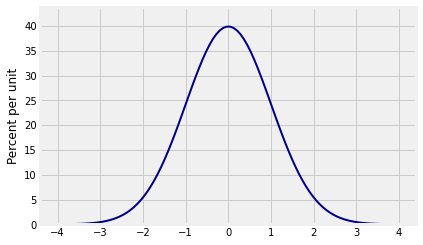
You can shade all the area to the left of a point , by providing the point as the right_end of the interval .
Plot_norm([-4, 4], 0, 1, right_end=1.5)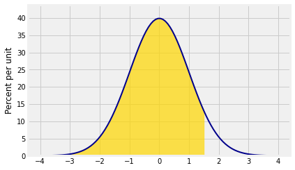
All the area to the right of a point:
Plot_norm([-4, 4], 0, 1, left_end=1.5)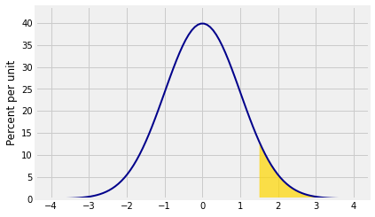
The area between two points:
Plot_norm([-4, 4], 0, 1, right_end=-1, left_end=1.5)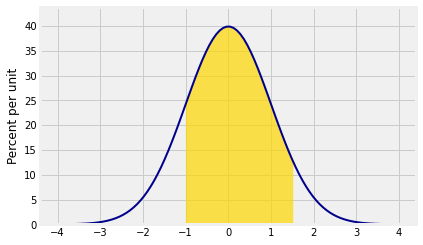
14.4.2 and 
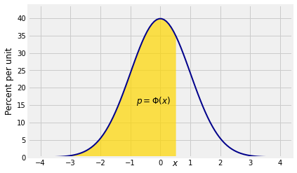
All the areas displayed above can be expressed in terms of the standard normal cdf .
Recall that the standard normal cdf is the function defined by
where is the standard normal curve.
For each , the value of is an area under the standard normal curve. The function takes a real number as its argument and returns a proportion which is all the area to the left of under the standard normal curve.
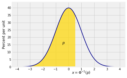
It will also be helpful to go the other way, and identify the such that is a specified value . In other words, we will need , the inverse of , which is determined by
For each in the interval , the value of is a point on the horizontal axis of the graph of the standard normal curve.
14.4.3 and in SciPy
As we noted in the previous section, there is no closed form formula for . So there also isn’t one for . But most computational systems provide excellent numerical approximations.
In SciPy the approximations are in the familiar stats module. For the standard normal cdf, use stats.norm.cdf just as you used stats.binom.cdf and so on. By default, stats.norm.cdf is based on the standard normal curve.
The area to the left of 1 under the standard normal curve:
stats.norm.cdf(1)0.8413447460685429The area between -1 and 1 under the standard normal curve can be found by using the cdf and subtraction in a familiar way:
stats.norm.cdf(1) - stats.norm.cdf(-1)0.6826894921370859In both examples above, we started with a point or points on the horizontal axis and used the cdf to find a related area. We can also go backwards, by specfiying an area and using to find a related point on the horizontal axis.
For example, if you want such that , you can use the percent point function stats.norm.ppf. The name comes from the expression “90% point” of the distribution, or equivalently, the 90th percentile.
stats.norm.ppf(0.9)1.2815515655446004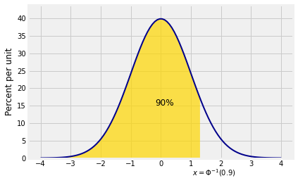
By the definition of an inverse, we should have . Let’s check that.
stats.norm.cdf(stats.norm.ppf(0.9))0.899999999999999914.4.4Example
Suppose the weights of a sample of 100 people are i.i.d. with a mean of 150 pounds and an SD of 20 pounds. Then the total weight of the sampled people is roughly normal with mean pounds and SD pounds.
Who cares about the total weight of a random group of people? Ask those who construct stadiums, elevators, and airplanes.
# Approximate distribution of total weight

n = 100
mu = 150
sigma = 20

mean = n*mu
sd = (n**0.5)*sigma

plot_interval = make_array(mean-4*sd, mean+4*sd)

Plot_norm(plot_interval, mean, sd)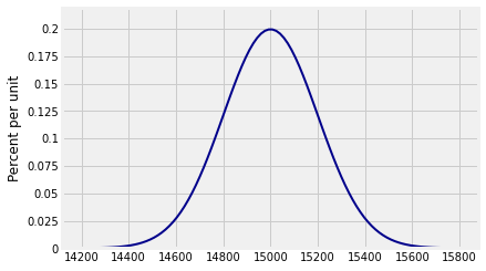
The chance that the total weight of the sampled people is less than 15,100 pounds is approximately the gold area below. The CLT allows us to use the normal curve as an approximation to the unknown exact distribution of the total weight.
Plot_norm(plot_interval, mean, sd, right_end=15100)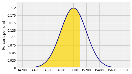
The function stats.norm.cdf takes the mean and SD as optional arguments. Remember that the names mean and sd were assigned in an earlier cell. Also remember that the answer below is not exact but an approximation based on the CLT.
stats.norm.cdf(15100, mean, sd)0.6914624612740131To find the approximate 90th percentile of the distribution of weights, you can use stats.norm.ppf with the mean and SD as arguments.
stats.norm.ppf(0.9, mean, sd)15256.31031310892The conclusion is where denotes the total weight.
14.4.5Using Standard Units
While it convenient to be able to enter the mean and SD as arguments to stats.norm.cdf and stats.norm.ppf, the fundamental curve is the standard normal curve. All the others are obtained by linear transformations.
Therefore all the calculations above can be done in terms of the standard normal cdf by standardizing, and therefore all normal approximations can (and will) be written in terms of the standard normal cdf . We don’t need to use a different cdf for each mean and SD.
For example, we can redo the two calculations above as follows.
To find the approximate chance that the total weight is less than 15100 pounds, first standardize 15100 and then use the standard normal cdf:
The calculation gives the same answer as before.
z = (15100 - mean)/sd

stats.norm.cdf(z) 0.6914624612740131To find 90th percentile of the approximate distribution of the , first find the 90th percentile of the standard normal curve. This value is the 90th percentile of any normal curve, measured in standard units.
z = stats.norm.ppf(0.9)
z1.2815515655446004Now convert the standard units back to pounds. The 90th percentile of the distribution of is approximately . The numerical answer is the same as before.
x = z*sd + mean
x
15256.31031310892