Odds Ratios - Data 140 Textbook

# HIDDEN
from datascience import *
from prob140 import *
import numpy as np
import matplotlib.pyplot as plt
plt.style.use('fivethirtyeight')
%matplotlib inline
from scipy import stats

Binomial $(n, p)$ probabilities involve powers and factorials, both of which are difficult to compute when $n$ is large. This section is about simplifying the computation of the entire distribution. The result also helps us understand the shape of binomial histograms.

from IPython.display import YouTubeVideo
YouTubeVideo("-5suvosCTCE")

Loading...

6.5.1Consecutive Odds Ratios¶

Fix $n$ and $p$ , and let $P(k)$ be the binomial $(n, p)$ probability of $k$ . That is, let $P(k)$ be the chance of getting $k$ successes in $n$ independent trials with probability $p$ of success on each trial.

The idea is to start at the left end of the distribution, with the term

P(0) ~ = ~ (1-p)^n

Then we will build up the distribution recursively from left to right, one possible value at a time.

To do this, we have to know how the probabilities of consecutive values are related to each other. For $k \ge 1$ , define the $k$ th consecutive odds ratio

R(k) = \frac{P(k)}{P(k-1)}

These ratios help us calculate $P(k)$ recursively.

\begin{align*} P(0) &= (1-p)^n \\ \\ P(1) &= P(0) \cdot \frac{P(1)}{P(0)} = P(0)R(1) \\ \\ P(2) &= P(1)R(2) \end{align*}

and so on.

Even though we already have a formula for the binomial probabilities, building the distribution using consecutive ratios is better computationally and also helps us understand the shape of the distribution.

YouTubeVideo("F8lx8OmLsXE")

Loading...

6.5.2Binomial Consecutive Odds Ratios¶

How is this more illuminating than plugging into the binomial formula? To see this, fix $k \ge 1$ and calculate the ratio $R(k)$ .

\begin{align*} R(k) &= \frac{\binom{n}{k}p^k(1-p)^{n-k}} {\binom{n}{k-1}p^{k-1}(1-p)^{n-k+1}} \\ \\ &= \frac{n-k+1}{k} \cdot \frac{p}{1-p} ~~~ \text{(after cancellation)} \end{align*}

Notice that the formulas for $R(k)$ are simple. This makes it easy to compute $P(k)$ recursively. For example, if $n \ge 3$ , we can compute $P(3)$ as

P(3) = (1-p)^n \big( \frac{n - 1 + 1}{1} \cdot \frac{p}{1-p} \big) \big( \frac{n - 2 + 1}{2} \cdot \frac{p}{1-p} \big) \big( \frac{n - 3 + 1}{3} \cdot \frac{p}{1-p} \big)

Answer

Multiply by $\frac{61-36}{36}\cdot 2$ to get 0.05844381950532852.

6.5.3Shapes of Binomial Histograms¶

Now observe that comparing $R(k)$ to 1 tells us whether the histogram is going up, staying level, or going down at $k$ .

\begin{align*} R(k) > 1 &\iff P(k) > P(k-1) \\ R(k) = 1 &\iff P(k) = P(k-1) \\ R(k) < 1 &\iff P(k) < P(k-1) \end{align*}

Note also that the form

R(k) = \big( \frac{n+1}{k} - 1 \big) \cdot \frac{p}{1-p}

tells us the the ratios are a decreasing function of $k$ . In the formula, $n$ and $p$ are the parameters of the distribution and hence constant. It is $k$ that varies, and $k$ appears in the denominator.

This implies that once $R(k) < 1$ for some $k$ , it will remain less than 1 for all larger $k$ . In other words, once the histogram starts going down, it will keep going down. It cannot come back up again.

That is why binomial histograms are either non-increasing or non-decreasing, or they go up and come down. But they can’t look like waves on the seashore. They can’t go up, come down, and go up again.

YouTubeVideo("--V_Z2QBc4w")

Loading...

Let’s visualize this for a $n = 23$ and $p = 0.7$ , two parameters that have no significance other than being our choice to use in this example.

n = 23
p = 0.7
k = range(n+1)
bin_23_7 = stats.binom.pmf(k, n, p)
bin_dist = Table().values(k).probabilities(bin_23_7)
Plot(bin_dist)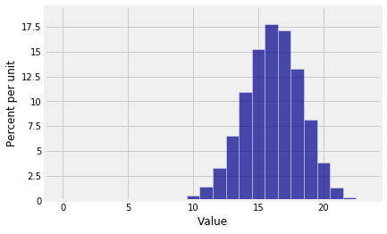

<matplotlib.figure.Figure at 0x10f4a5780>

# It is important to define k as an array here,
# so you can do array operations
# to find all the ratios at once.
k = np.arange(1, n+1, 1)
((n - k + 1)/k)*(p/(1-p))

array([53.66666667, 25.66666667, 16.33333333, 11.66666667,  8.86666667,
        7.        ,  5.66666667,  4.66666667,  3.88888889,  3.26666667,
        2.75757576,  2.33333333,  1.97435897,  1.66666667,  1.4       ,
        1.16666667,  0.96078431,  0.77777778,  0.61403509,  0.46666667,
        0.33333333,  0.21212121,  0.10144928])

What Python is helpfully telling us is that the invisible bar at 1 is 53.666... times larger than the even more invisible bar at 0. The ratios decrease after that but they are still bigger than 1 through $k = 16$ . The histogram rises till it reaches its peak at $k = 16$ . You can see that $R(16) = 1.1666 > 1$ . Then the ratios drop below one, so the histogram starts going down.

6.5.4Mode of the Binomial¶

A mode of a discrete distribution is a possible value that has the highest probability. There may be more than one such value, so there may be more than one mode.

We have seen that once the ratio $R(k)$ drops below 1, it stays below 1, so the histogram keeps falling. To identify the mode, therefore, we will find all values of $k$ such that $R(k) \ge 1$ .

Let $q = 1-p$ . Every value $k$ for which $R(k) \ge 1$ must satisfy

\big( \frac{n+1}{k} - 1 \big) \frac{p}{q} ~ \ge ~ 1

That is,

\frac{n+1}{k} ~ \ge ~ \frac{q}{p} + 1 ~ = ~ \frac{1}{p}

which is equivalent to

k ~ \le ~ (n+1)p

We have shown that for all $k$ in the range 0 through the integer part of $(n+1)p$ , the histogram rises; for larger $k$ , it falls.

Therefore the peak of the histogram is at the largest $k$ in this range. That’s the integer part of $(n+1)p$ .

So the integer part of $(n+1)p$ is a mode of the binomial.

Because the odds ratios are non-decreasing in $k$ , the only way in which there can be more than one mode is if there is a $k$ such that $R(k) = 1$ . In that case, $P(k) = P(k-1)$ and therefore both $k$ and $k-1$ will be modes. To summarize:

The mode of the binomial $(n, p)$ distribution is the integer part of $(n+1)p$ . If $(n+1)p$ is an integer, then $(n+1)p - 1$ is also a mode.

To see that this is consistent with what we observed in our numerical example above, let’s calculate $(n+1)p$ in that case.

(n+1) * p

16.799999999999997

The integer part of $(n+1)p$ is 16, which is the mode that we observed.

But in fact, $np$ is a more natural quantity to calculate. For example, if you are counting the number of heads in 100 tosses of a coin, then the distribution is binomial $(100, 1/2)$ and you naturally expect $np = 50$ heads. You don’t want to be worrying about $101 \times (1/2)$ .

In fact you don’t have to worry when $n$ is large, because then $np$ and $(n+1)p$ are pretty close. In a later section we will examine a situation in which you can use $np$ to get an approximation to the shape of the binomial distribution when $n$ is large.

6.5 Odds Ratios

6.5.1Consecutive Odds Ratios¶

6.5.2Binomial Consecutive Odds Ratios¶

6.5.3Shapes of Binomial Histograms¶

6.5.4Mode of the Binomial¶